Read Depth vs. Coverage vs. Breadth: Sequencing Metrics That Get Used Interchangeably

A major, recurring source of confusion in secondary sequencing analysis is the loose, interchangeable use of core quality control metrics. In peer-reviewed publications and pipeline reports, researchers frequently write “30x coverage” or “depth of 30x” as if they are the identical measurement, and occasionally conflate these with “95% of the target genome covered.”

This loose terminology is a significant problem. Read depth, fold coverage, and breadth of coverage are three mathematically distinct parameters that describe different aspects of a sequencing run’s data distribution. Treating them as interchangeable black-box values masks local position-to-position variability, hides systematic sequencing gaps, and can lead to over-confident variant classifications at poorly covered loci.

This article serves as a definitive, technically precise reference guide, defining each metric mathematically, exploring where they decouple, and outlining why reporting them distinctly is essential for rigorous sequencing quality control.

---

The Sequencing Metrics Matrix

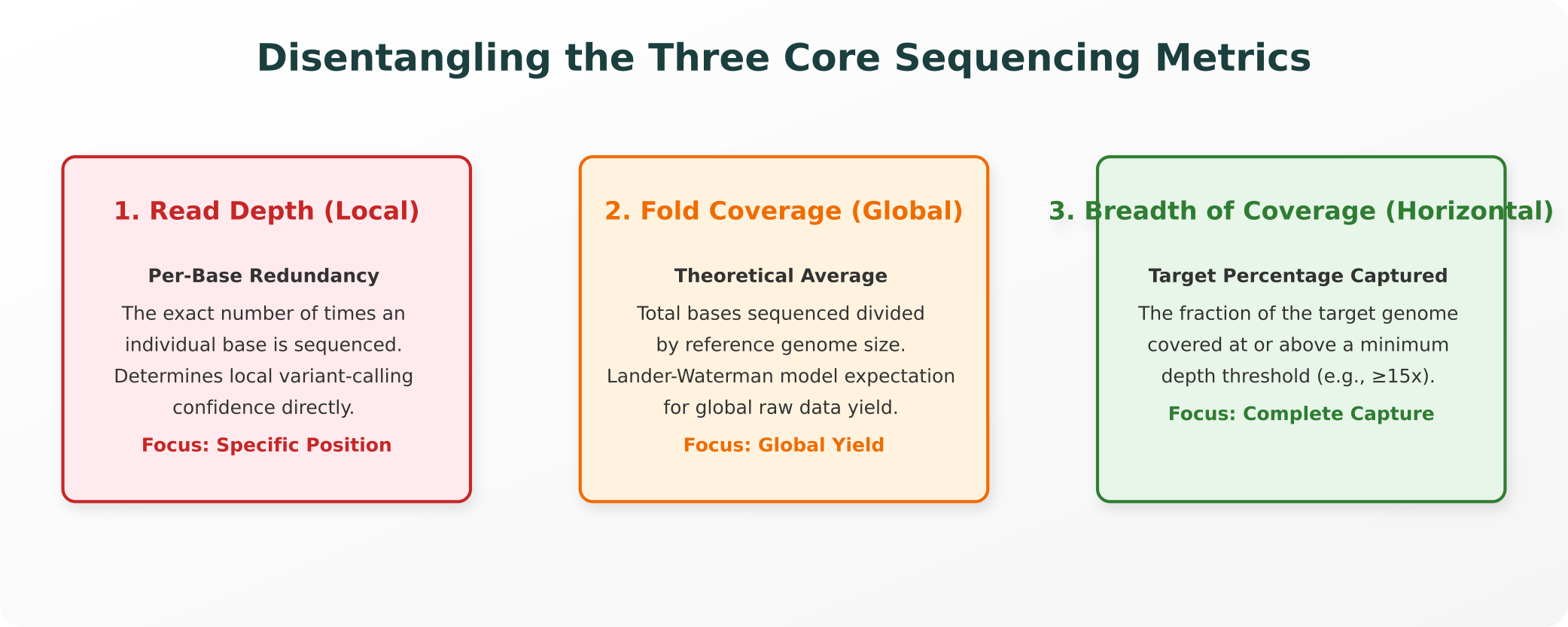
These three core metrics describe connected but mathematically distinct dimensions of a sequencing run’s data yield and distribution:

---

1. Read Depth: Per-Position Redundancy

Read depth (commonly termed depth of coverage or raw depth) is a local, position-level metric.

• What It Is: The exact number of individual sequencing reads that physically overlap and map to a specific nucleotide coordinate in your reference alignment file (BAM or CRAM).
• The Calculation: If twenty distinct reads cover the coordinate chr1:10,000, the local read depth at that specific locus is exactly 20x. Tools like samtools depth parse through alignment files to compute this value for every individual base.
• Why Averaging Masks Variability: While pipelines often report an average read depth across a genome (e.g., “average depth of 30x”), this average can hide enormous, biochemically driven variation. Due to GC-bias, repetitive elements, or capture inequalities in targeted sequencing, some loci might have 150x depth while others have 0x, meaning the average tells you nothing about the data’s true local distribution.

---

2. Fold Coverage: The Theoretical Global Expectation

Fold coverage (frequently termed raw genomic coverage or average coverage) is a global, run-wide metric of total data yield.

• The Calculation: Fold coverage is calculated using a standard, lander-waterman-style formula:

$$C = \frac{L \times N}{G}$$

Where:

• $L$ is the average length of a sequencing read (in base pairs).

• $N$ is the total number of reads generated during the run.

• $G$ is the length of the reference target genome (e.g., approximately 3.2 billion base pairs for humans).

• A Theoretical Expectation: If you sequence a human genome and generate 96 gigabases of raw data, your global fold coverage is exactly 30x ($96 \times 10^9$ / $3.2 \times 10^9$). However, because sequencing is a stochastic process governed by Poisson distribution, a fold coverage of 30x does not mean that every base was read exactly 30 times. According to the Lander-Waterman model, some bases will naturally be read far more frequently, while others will remain completely unsequenced.

---

3. Breadth of Coverage: The Horizontal Metric

Breadth of coverage (commonly termed horizontal coverage) is a percentage-based target metric.

• What It Measures: The proportion of the target reference genome (or targeted panel regions, such as the exome) that is covered by at least a specified minimum number of overlapping reads.
• The Format: It is always reported as a percentage paired with a minimum depth threshold (e.g., “98.5% of target bases covered at $\ge$ 15x”).
• The Difference: While read depth tells you how many times a base was read (vertical confidence), and fold coverage tells you the average redundancy of your total raw data (theoretical expectation), breadth of coverage tells you how much of the genome you actually sequenced at all (horizontal completeness).

---

Where Conflation Causes Practical Failures

In high-throughput genomics, relying on a single, averaged metric to represent all three dimensions introduces critical blind spots:

• The High-Depth, Low-Breadth Trap: A targeted exome capture run can yield an impressive “average depth of 100x.” However, if the capture probe library was poorly optimized or had high GC-content bias, 30% of the target exome might have 0x coverage, while the remaining 70% was sequenced to over 140x depth. Citing only the 100x average depth masks the fact that nearly a third of your target genes were completely missed, representing poor breadth of coverage.
• False Variant Calling Confidence: A variant calling algorithm’s statistical confidence at a specific genomic coordinate depends entirely on the local read depth at that locus (and the ratio of reference to alternative alleles), not on the run-wide fold coverage. If a paper cites “30x coverage” globally, but the target variant locus only has a local read depth of 2x due to alignment issues, calling a heterozygous mutation at that locus is highly likely to be a sequencing artifact.
• Incomplete Target Captures: In clinical diagnostics, missing a single gene due to low local breadth of coverage can lead to false-negative diagnoses for rare genetic conditions. Clinicians must know exactly what fraction of the target panel was covered at a diagnostic-grade threshold (e.g., $\ge$ 20x), making breadth of coverage the absolute priority metric.

---

Best Practices for Quality Control Reporting

To ensure data reproducibility and absolute scientific integrity, research teams should adopt several reporting habits in their methodologies and QC reports:

1. Report the Metrics Separately: Never write “30x coverage” in isolation. Always specify the average fold coverage (based on total data yield), the average read depth, and the breadth of coverage at clinically relevant thresholds (e.g., “the target was sequenced to a mean read depth of 35x, with 97.2% of targeted bases covered at $\ge$ 15x”).
2. Utilize Standardized QC Software: Use established, peer-reviewed computational tools (such as Picard CollectHsMetrics, Qualimap, or Samtools coverage) to systematically calculate and plot these parameters.
3. Inspect Local Depth Variance: Always generate and inspect coverage-distribution histograms or local depth plots across your target genes of interest to identify systematic sequencing gaps or capture failures before trusting called variants.

---

References and Authoritative Specifications

For computational biologists seeking to review the mathematical models and software specifications discussed, the following resources serve as primary references:

1. The Lander-Waterman Model: Lander, E. S., & Waterman, M. S. (1988). “Genomic mapping by fingerprinting random clones: a mathematical analysis.” Genomics, 2(3), 231-239. doi:10.1016/0888-7543(88)90007-9
2. Samtools Coverage Specifications: Heng Li et al. (2009). “The Sequence Alignment/Map format and SAMtools.” Bioinformatics, 25(16), 2078-2079. doi:10.1093/bioinformatics/btp352
3. Picard CollectHsMetrics Documentation: Broad Institute’s standard utility for evaluating target-enrichment sequencing runs. broadinstitute.github.io/picard
4. Qualimap QC Tool: Okonechnikov, K. et al. (2016). “Qualimap 2: advanced multi-sample quality control for high-throughput sequencing data.” Bioinformatics, 32(2), 292-294. doi:10.1093/bioinformatics/btv566